Alternative Investments & Pension Funds

We define you purchasing

and selling Brent strategy

Institutional

BUSINESS CASE

Analysis of a management model with Brent Options

OBJECTIVE: Purchase optimization, coverage improvement and risk control

Hypothesis

Functional analysis

Qualitative and Quantitative Analysis Considerations

Model Risk Matrix

Volatility parameterization

Model Risk scenario parametrization

Monthly Historical Volatility Chart

STRATEGY, conclusions and tactical part

Observations

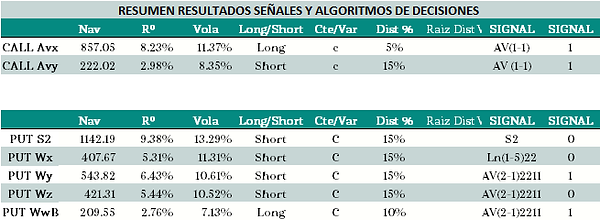
Parameterization analysis

Results Matrix

High Volatility Vs Low Volatility. Moledo Waves of Volatility

1. Variable choice of Volatility risk factors

Volatility Spreads (high-low)

2. Selection of parameters (independent variables)

Parameters quantitative analysis
% Pending variation of the Volatility waves (How, When and Where)

3. Selection of systematization factors

Time and moneyness; Vola Risk factor
Volatility and spreads of Volatility differential

4. Selection Model Analysis Criteria

Failure evaluation -What if scenarios
Model stress test
Error rulling
Reassessment of scenarios for acceptable volatility limits.

Data

Since 1995. Brent, Gasoline and Diesel
Brent and Gasoil implied volatility data
Crude Oil Volatility Indices, OVX since 2007

Parameterization.

Definition of an initial model as the basis for evaluating seasonal and/or specific risks based on criteria of volatility and movements of the underlying.
Definition of variables for risk parameterization, underlying prices, volatility and time
Introduction of quantitative risk limit signals. Second level.
Simulation of adjustments of inputs of second level variables of signals on risk variables.
Data analysis and results of the model by results of the risk/return binomial and adjustments on the purchase program.

Correlation analysis of Brent with Diesel and Gasoline
In the studies of relative behavior between oil and its derivatives, diesel oil and gasoline, we discovered that the symmetry of the correlation is much better in the correlation analysis of minimum and maximum prices of the day, but not in openings and closings.
Market liquidity. Fork width and price slippage.
Operational risk assessment.
Definition and analysis of the mechanisms for hedging, neutralization or exit of positions.
Quantitative risk assessment, kurtosis, skewness and drawdown.

Model specific parameterization. Ex ante.

Operation with options at 60 - 90 days to expiration and systematization of the rolls before expiration.
The model includes a matrix of Delta, Gamma and Vega as risk management parameters.
Strike price distance (moneyness) based on risk criteria parameterized by Volatility in the back-testing simulator. Independent variables.
Introduction of volatility signals defined by the Model's risk matrix. Independent variables.
Definition of the operational rules of the Model. Independent and dependent.
The Model includes a matrix of "what if" scenarios for the valuation analysis and hypotheses of probable risk scenarios.

We take two values for the parameterization, firstly the data on the volatility of ATM Calls and Puts (since 1995) and the OVX Volatility Index.
Volatility smile parameterized in the simulator and introduced as a variable to create hypotheses in the change of the curve and Volatility smirk
We segment the signals into minimum and maximum volatility for periods of 11, 22, 44 and 66 sessions, looking for risk differences that allow us to reduce the volatility of the model itself.
We analyze the volatility amplitude spread (differential) between highs and lows, based on the following hypothesis:
- When the volatility spread between minimums and maximums widens, we interpret a risk scenario with a probability of a rise in volatility.
- When the volatility spread between minimums and maximums narrows, we interpret a scenario of a greater probability of a decline in volatility.
- We include the volatility spread as a variable of amplitude over time in the simulation, which allows us to optimize the parameterization of the Volatility behavior patterns.
- The Model introduces the Volatility Smile parameterizing curvature, slope and smirk.

Situations of extreme volatility (Jumps in volatility.
Analysis of volatility jumps (Slope of the Volatility curve)
Strategy exit affected by volatility in a range greater than x%
Systematize tactical coverage when there is a jump greater than y%

Observations:

Of the models evaluated, the use of amplitudes in volatility time and calculation of the volatility angle obtained better results in almost all the models except in S2 (spreads in % of maximum and minimum volatility).

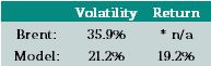
The graph shows the comparison of the historical Volatility of the Model against the historical Volatility of Brent in monthly periods of 22 sessions.

From the work carried out and the simulations, we can conclude in a first phase that the application of the proposed volatility model obtains very satisfactory results, with high risk control, improving profitability.

The strategies with which we will work the simulation period in real, will be: Mariposa/Condor, Diagonal Calendar Spreads, Sell - Buy Call and Sell - Buy Put

Operational Criteria applied in the Model:

a) Definition of Strikes based on moneyness (distance to the underlying)

b) Options with maturities of 3 months and 2 months (composition calendar spreads

c) Closing of positions at 30 days of expiration

d) Simulation in carrying to expiration ¿??. Test and risk assessment.

e) Tactical strategy of introducing purchase of Call and purchase of Put at higher expiration

(1 or 2 years) seeking anticipation of market risks or strong price fluctuations.

By systematic coverage tactic

By macro price risk hedging tactic

The behavior of the market is lognormal in its distribution.
Leptokurtic market, more ups than downs.
Persistence in the bearish trend of the market.
There is an interrelation between the rise in volatility and the rise in the market (Pstv. Volatility jumps).
Existence of price patterns in sections with trends.

Notes. Observations on the Model: